Topics

Artificial Intelligence

Privacy in Azure ML

corifeanu

Rating & reviews (0 reviews)

Study Notes

Data science projects, including machine learning projects, involve analysis of data; and often that data includes sensitive personal details that should be kept private.

Differential privacy
Technique that is designed to preserve the privacy of individual data points by adding "noise" to the data. The goal is to ensure that enough noise is added to provide privacy for individual values while ensuring that the overall statistical makeup of the data remains consistent, and aggregations produce statistically similar results as when used with the original raw data.

The noise is different for each analysis, so the results are non-deterministic – in other words, two analyses that perform the same aggregation may produce slightly different results.
The amount of variation caused by adding noise is configurable through a parameter called epsilon

A low epsilon value provides the most privacy, at the expense of less accuracy when aggregating the data.
A higher epsilon value results in aggregations that are more true to the actual data distribution, but in which the individual contribution of a single individual to the aggregated value is less obscured by noise.

Dataaggregation
A machine learning project typically involves an iterative process of data analyses in order to gain insights into the data and determine which variables are most likely to help build predictive models.

Analyzing data usually involves aggregative and statistical functionsthat provide insights into the statistical distributionof variables and the relationships between them. With large volumes of data, the aggregations provide a level of abstraction; but with smaller amounts of data, or with repeated analyses, even aggregated results may reveal details about individual observations.

To run the experiment you need opendp-smartnoise

pip install opendp-smartnoise==0.1.4.2

Load data

import pandas as pd

data_path = 'data/diabetes.csv'
diabetes = pd.read_csv(data_path)
diabetes.describe()

Perform analysis.

import opendp.smartnoise.core as sn

cols = list(diabetes.columns)
age_range = [0.0, 120.0]
samples = len(diabetes)

with sn.Analysis() as analysis:
# load data
data = sn.Dataset(path=data_path, column_names=cols)

# Convert Age to float
age_dt = sn.to_float(data['Age'])

# get mean of age
age_mean = sn.dp_mean(data = age_dt,
privacy_usage = {'epsilon': .50},
data_lower = age_range[0],
data_upper = age_range[1],
data_rows = samples
)

analysis.release()

# print differentially private estimate of mean age
print("Private mean age:",age_mean.value)

# print actual mean age
print("Actual mean age:",diabetes.Age.mean())

Result:
Private mean age: 30.192
Actual mean age: 30.1341

Quite good.

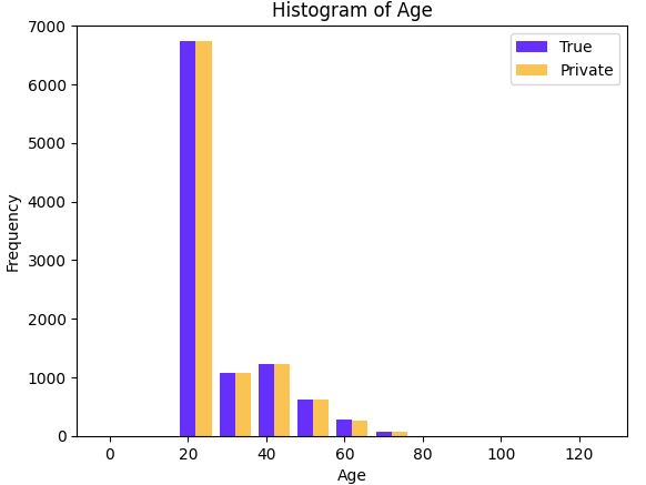
Compare age (with noisy and real)

import matplotlib.pyplot as plt

with sn.Analysis() as analysis:
data = sn.Dataset(path = data_path, column_names = cols)

age_histogram = sn.dp_histogram(
sn.to_int(data['Age'], lower=0, upper=120),
edges = ages,
upper = 10000,
null_value = -1,
privacy_usage = {'epsilon': 0.5}
)

analysis.release()

plt.ylim([0,7000])
width=4
agecat_left = [x + width for x in ages]
#agecat_right = [x + 2*width for x in ages]
plt.bar(list(range(0,120,10)), n_age, width=width, color='blue', alpha=0.7, label='True')
plt.bar(agecat_left, age_histogram.value, width=width, color='orange', alpha=0.7, label='Private')
plt.legend()
plt.title('Histogram of Age')
plt.xlabel('Age')
plt.ylabel('Frequency')
plt.show()

print(age_histogram.value)